

Lite Classify
by LeoBar · a lightweight desktop app for object-based land-cover mapping of drone orthomosaics
User manual
Turn a drone orthomosaic into a checked land-cover map
Lite Classify splits an aerial image into objects, describes each one by its colour, texture, shape, height and appearance, helps you find the classes the scene really contains, learns those classes from examples you click, and checks the finished map against an independent sample. This manual walks one real -hectare survey through every step: objects, nine classes, training objects and independently labelled check points.
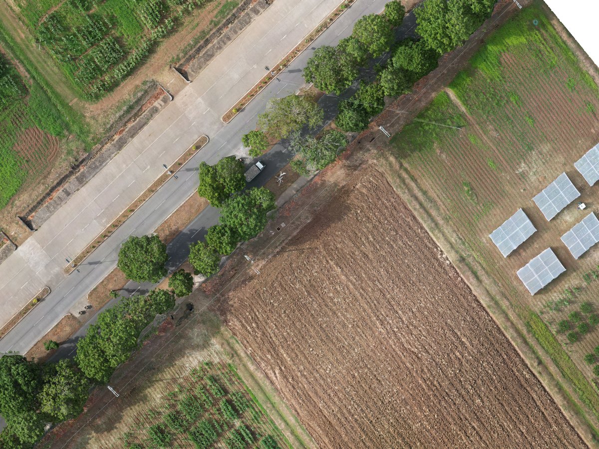
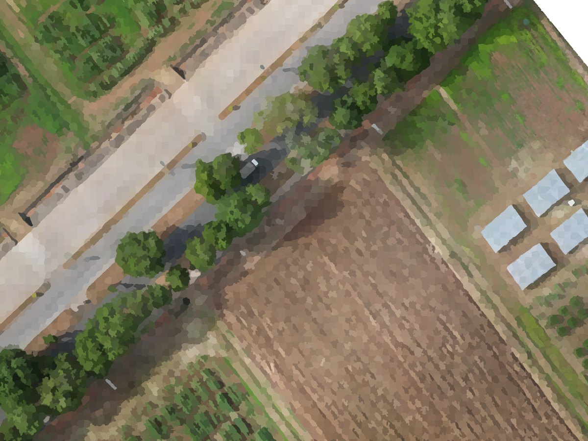
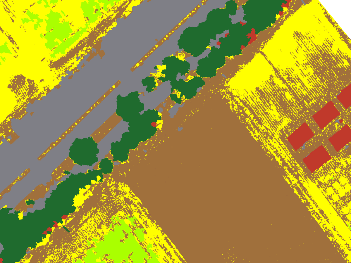
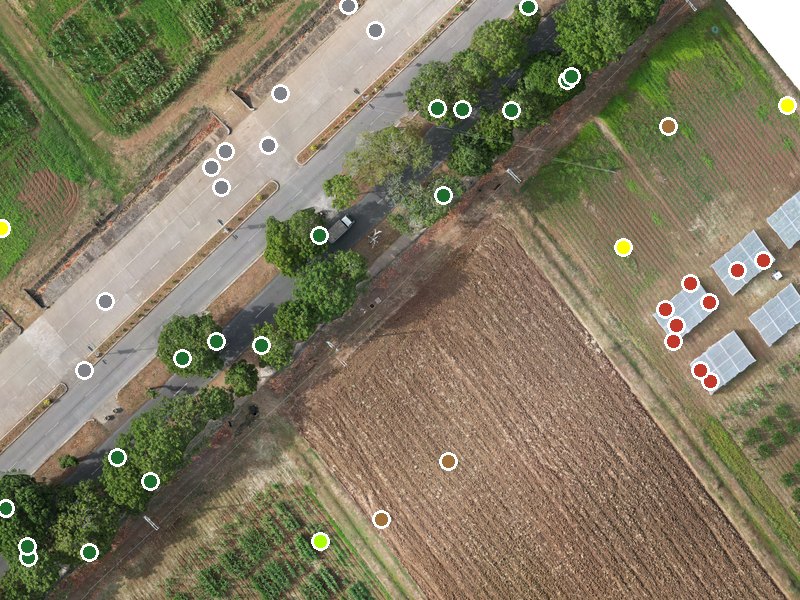
- Bare
- Crop 1
- Crop 2
- Grass
- Water
- Tree
- Road
- Building
- Mud
Getting started
Install, meet the worked example, learn the window.
Part BHow it works
Segments, the 24 measurements, DINOv2 appearance, class discovery, Random Forest, accuracy.
Part CWorkflow
Every control in the four tabs, step by step.
Part DReference
Files, parameters, troubleshooting, glossary, licence and citation.
1Welcome
Lite Classify is a desktop tool for geographic object-based image analysis (GEOBIA) of very-high-resolution drone imagery. It was built to map land cover in tropical landscapes, from canopy gaps and restoration patches to farms and campuses, and it works for any cover types you can recognise by eye in an RGB orthomosaic: trees, crops, grass, bare ground, roads, buildings, water.
Lite Classify picks up where Lite Flight leaves off. Plan and fly the survey with Lite Flight, process the photos into an orthomosaic and surface model in your photogrammetry software, then bring both into Lite Classify to map them. It is one self-contained program that runs offline on a single workstation, with no Python, GIS software, account or internet connection needed.
You work through four tabs, left to right. Each tab hands its result to the next.
Computing is the quick part. On the worked example, segmentation and feature measurement for objects ran in minutes on a desktop GPU. Most of your time goes into reviewing groups, labelling examples and checking the result.
2Installing and launching
Free and open source. Lite Classify is released under the GNU General Public License v3 (see Part D, 17). Download the installers from the GitHub release page (mirror on Google Drive); the source code is on GitHub.
Lite Classify ships as a self-contained Windows program; you do not need Python or any GIS software installed.
- Download an installer from the release page, or from the Google Drive mirror. Setup CPU (about 320 MB) runs on any Windows 10/11 PC. Setup GPU (about 1.8 GB) adds NVIDIA CUDA support: much faster segmentation and appearance features on an NVIDIA graphics card. Both work offline once installed.
- Run the installer. It installs for your user account, with no administrator rights needed, into
%LOCALAPPDATA%\Programs\Lite Classify, and adds a Start-menu shortcut (a desktop shortcut is optional). Installing one edition over the other replaces it. Uninstall from Windows Settings › Apps. - Start Lite Classify from the Start menu. A splash screen shows while the libraries load; the first launch can be slow, later launches are quicker.
- Check the console at the bottom of the window. It should say
Load an image to begin.Every action the app takes is logged there, including errors. - Check the Segmentation Engine box on Tab 1. If GPU is selectable, an NVIDIA CUDA graphics card was found; segmentation and the DINOv2 appearance features will run on it. If it is greyed out, everything runs on the CPU, just slower.
Running from source instead
Clone the repository, create a Python 3.13 environment (python -m venv .venv), run pip install -r requirements.txt, then python liteclassify.py. The requirements pull the CUDA 12.4 build of PyTorch; on a machine without an NVIDIA GPU, use requirements-cpu.txt instead. The DINOv2 weights (dinov2_vits14_pretrain.pth, about 85 MB) are downloaded once on first use, or read from a models folder beside the code. Close the app before upgrading packages: Windows locks loaded libraries.
Optional: DINOv3 appearance features
Lite Classify ships with DINOv2 for its appearance features. It can also use Meta's DINOv3 ViT-S+/16, which in our tests grouped look-alike objects more sensibly. DINOv3 is under Meta's own licence, so it is never bundled or downloaded by the app: request the weights from Meta (github.com/facebookresearch/dinov3), then pick the file under Backbone in Tab 2 (Part C, 8.1). Only the ViT-S+/16 file (dinov3_vits16plus_pretrain_lvd1689m-….pth) is accepted; the app checks the file's checksum against its name.
| Requirement | Needed | Notes |
|---|---|---|
| Operating system | Windows 10 or 11, 64-bit | On a fresh machine you may need the Microsoft Visual C++ Redistributable (x64). |
| Graphics card | Optional | An NVIDIA GPU with CUDA speeds up segmentation (about 10× in our tests) and the DINOv2 appearance features. |
| Memory (RAM) | 16 GB or more recommended | Lite Classify checks memory before loading, resampling and segmenting, and suggests a coarser resolution or tiling when a step would not fit. Very large mosaics are read at reduced resolution on load. |
| WebODM | Optional | Only to make orthomosaics from drone photos inside Lite Classify (Part C, 6.1). Installed and run separately; Lite Classify includes no photogrammetry. |
| Disk | Room for a workspace | Each orthomosaic gets a <name>_workspace folder next to it. A processed extent gets its own folder (Part C, 6.5). |
3The worked example
Every figure and number in this manual comes from one drone survey: the ha CAFS experimental agricultural site of the University of the Philippines Los Baños, used for field experiments in agriculture-related courses. It lies along UPLB Pili Drive in Los Baños, Laguna, northeast of the Mount Makiling Forest Reserve and outside its boundaries. In one flight it holds what an agricultural map has to separate: annual crops in rows and blocks, thin grass strips between bare beds, dying grass that is nearly the colour of soil, mud, a pond and ditches, a road lined with trees, and buildings.
- Orthomosaic
- RGB, 8-bit, cm/px
- Native size
- × px
- Surface model
- DSM, cm/px
- Working grid
- 5 cm · × px
- Mapped area
- ha
- Coordinates
- WGS 84 / UTM 51N
- DSM heights
- – m
- Objects
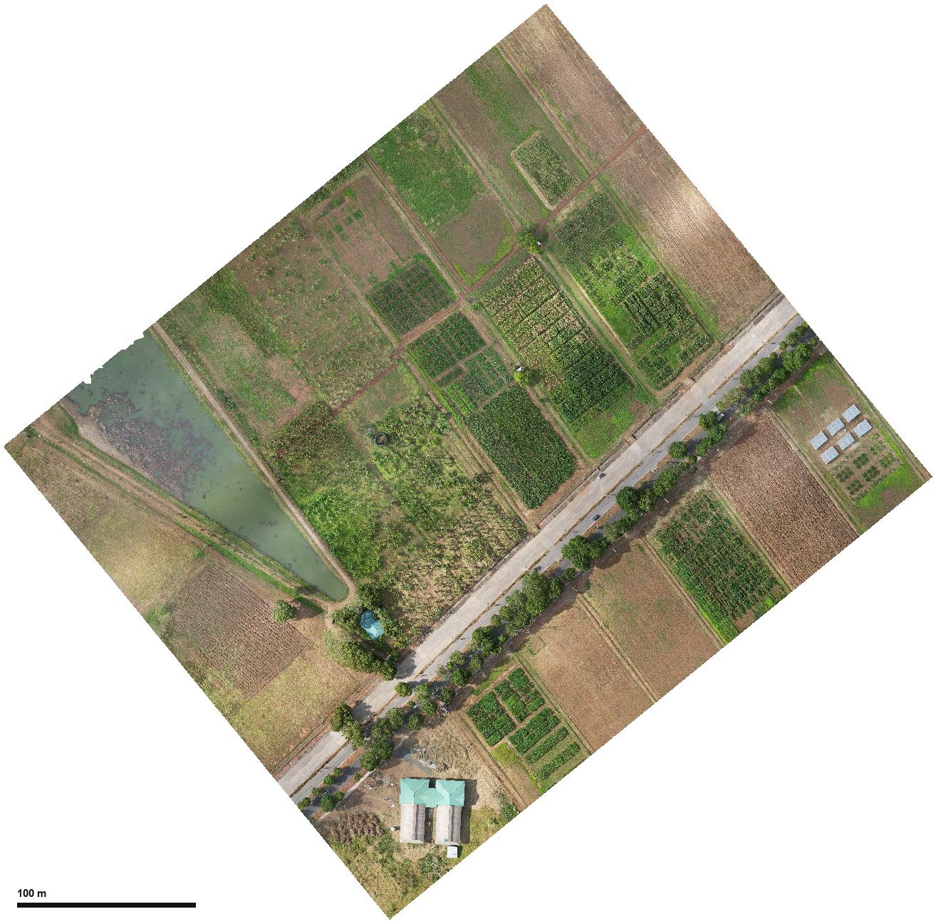
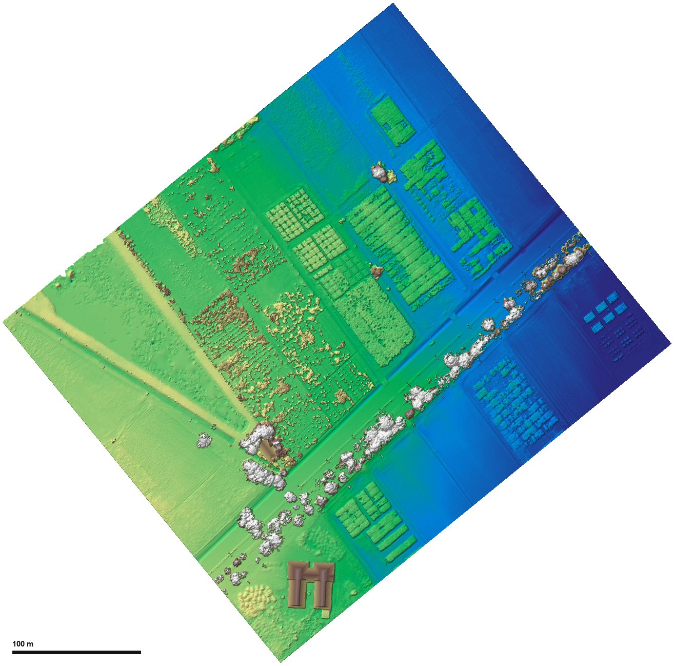
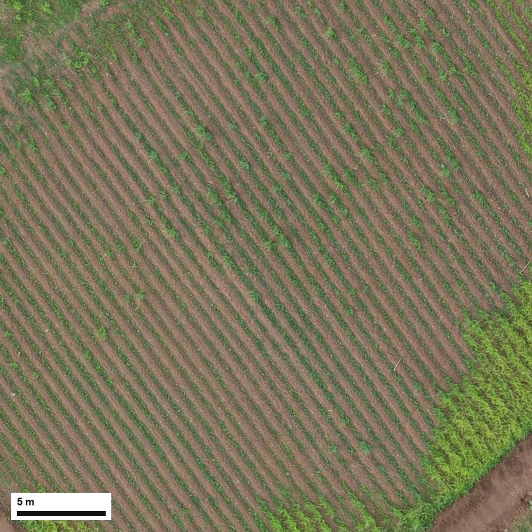
The orthomosaic was captured at about 2.2 cm per pixel. The worked example segments it on a 5 cm working grid into small objects, about 2 m² each, so that crop rows and beds stay separate, and adds the DINOv3 appearance features (Part B, 5.4). Grass strips narrower than an object are recovered after classification by the greenness refinement (Part B, 5.9). The DSM comes from the same photogrammetry run on a coarser grid; Lite Classify places it by its coordinates, so the two need not share a pixel size.
The sample data (orthomosaic, DSM and the saved workspace) can be downloaded from the sample-data folder on Google Drive, so you can follow every step on the same data.
4A tour of the interface
The window has a menu bar, four tabs, a control column on the left of each tab, a large map viewer, and a console strip along the bottom that logs every step. All four viewers share one copy of the image, so switching tabs is instant even on large mosaics, and they share the zoom and pan: switching tabs keeps the same view. The bar above each map shows the image's native and working resolution, size, coordinate system and bit depth; below that, the map coordinates under the cursor.
Menus
| Menu | Item | Shortcut | Does |
|---|---|---|---|
| File | New | Ctrl+N | Start a blank session. Asks first if there are unsaved changes. |
| Load Workspace… | Ctrl+O | Pick a _workspace folder and reopen everything in it. | |
| Save Workspace | Ctrl+S | Save the whole session beside the orthomosaic. | |
| Save Workspace As… | Ctrl+Alt+S | Copy the orthomosaic, DSM and workspace to a new folder and carry on from the copies. | |
| Import | Orthomosaic from Drone Photos (WebODM)… | Have your WebODM make the orthomosaic and DSM from a folder of drone photos, then load them (Part C, 6.1). | |
| Orthomosaic… | Same as Browse on Tab 1. | ||
| DSM… | Attach a surface model. | ||
| Ground Truth CSV… | Bring in field points for Tab 4. | ||
| About | Manual | Opens this manual. |
Closing the window, New and Load Workspace all ask Save / Discard / Cancel when there is unsaved work.
The four tabs
Load, View & Segment
Orthomosaic and DSM paths (or a link to make them from drone photos with WebODM), resampling, colour correction, the SLIC settings (with Colour/texture at for measuring finer than the segmentation grid), the engine, Run Segmentation, boundary and elevation overlays, and Process This Extent Only.
Discover Classes
Find Groups (with the DINOv2 or DINOv3 backbone), a list of group cards, a scrolling gallery of the selected group's tiles, naming, merge, split, ignore and find-similar tools, a group overlay on the map, and Send Named Groups to Classification.
Classification
Class list, the Map View (Ortho, Segments or Classified, with training samples, segment boundaries and opacity), selection, grow and merge tools, Check Class Separability, What to Label Next, Train, Greenness Refinement, Classify All Segments, the minimum mapping unit, and export.
Accuracy Assessment
Reference source (a ground-truth CSV, matched to your classes, or generated points), sampling design (simple random or stratified by map class), the point list with assign, unassign and delete tools, Save and Export Points, Run Accuracy Assessment, and the Iterations list of earlier runs.
Each tab is described control by control in Part C.
Mouse and keys
| Action | Where | What it does |
|---|---|---|
| Scroll wheel | Any viewer | Zoom in and out. Zoomed in, the viewer draws a sharp patch of the visible area. |
| Drag | Any viewer | Pan. |
| Click a group card; Ctrl/Shift+click | Tab 2 group list | Select one group; add groups or a range to the selection. |
| Click, Ctrl/Shift+click a tile | Tab 2 gallery | Select tiles. Right-click to move them to another group, a new group, or out of all groups. |
| Double-click a tile | Tab 2 gallery | Zoom the map to that segment and outline it. |
| Right-click a segment | Tab 2 map | Move it to a group or a new group, leave it out, or show its group. |
| Click an object | Tab 3 | Add it to the highlighted class as a training sample. Click again to remove it. |
| Ctrl + drag | Tab 3 | Paint: every object the cursor crosses joins the highlighted class. |
| Right-click an object | Tab 3 | Find Similar Segments, or Show Its Group in Discover. |
| Click (Selection Mode on) | Tab 3 | Select a seed; the Grow Tolerance slider then grows it. |
| Ctrl + Z | Tab 3, Selection Mode on | Undo the last selection change. |
| Double-click a class | Tab 3 class list | Rename it or change its colour. |
| Click a point | Tab 4 | Tick or untick it. |
| Right-click a point / empty map | Tab 4 | Assign a class, unassign, delete; or add a point here. |
| Ctrl + drag a point | Tab 4 | Move it. |
| , and . | Tab 4 | Previous and next point. |
| Double-click a row | Tab 4 point list / Iterations | Zoom to that point / show that iteration's results. |